4. Quick Intro

4.1 Simple Network Scenario

In this section we will show how to build, configure and simulate the following simple network topology:

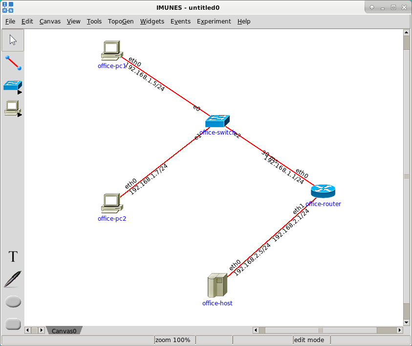
Personal computers (office-pc1 and office-pc2) from the network 192.168.1.0/24 are connected to the LAN switch (office-switch) which is connected to the router (office-router). The server (office-host) from the network 192.168.2.0/24 is directly connected to the router (office-router). Personal computers from the first network have route only to the network 192.168.2.0/24. The server from the second network has the default route. Quagga routing is enabled on the router in order to be able to serve and receive dynamic route updates.

4.1.1 Building a simple network

After running IMUNES on FreeBSD with some kind of X11 window manager (see Section 3), we will build previously described network using tools from the toolbox (see Section 3.1).

4.1.1.1 Adding and deleting network elements

To draw a node click on the corresponding node tool and then click on the workspace to place it. To connect nodes click on the Link tool, then click and hold on the source node and go to the destination node.

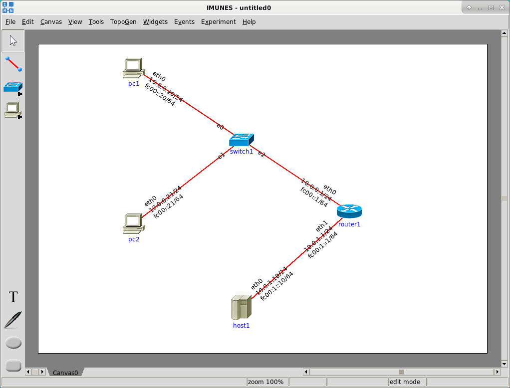
Now draw a router, a host, a LAN switch and two PCs. Using the Link tool connect the LAN switch to the router and then connect each PC to the LAN switch. Connect the host directly to the router. The created network topology should look like the one in Figure 4.1.

Figure 4.1: Simple network topology

When nodes are connected with the Link tool (the direction does not matter), the source node, the destination node and the link automatically get preconfigured parameters. When a mouse pointer is above a node or a link, some of the configured parameters are shown on the left side of the statusbar placed at the bottom of the window (Figure 4.2).

Figure 4.2: Node parameters in the statusbar

Some of the parameters can be visible on the canvas: interface names (link layer: e0, e1, e2 and network layer: eth0, eth1), IPv4/IPv6 addresses of network layer elements (PC, host, router), node names (router1, host1, switch1, pc1, pc2) and link labels (Bandwidth, Delay, BER or Duplicate if their values are not default).

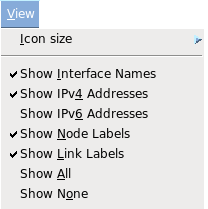
You can manipulate with the visibility of nodes and links parameters from the View menu (Figure 4.3). In this simple scenario we do not want for IPv6 addresses to be visible, so we will turn the Show IPv6 Addresses option off.

Figure 4.3: Show or hide nodes and links parameters

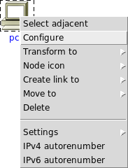
To delete the network element select it using the Select tool and then use the Delete keyboard button. You can also delete it by right clicking on it and clicking on the Delete label in the popped up menu. The node deletion is automatically followed by the deletion of associated links.

4.1.1.2 Rearranging network elements

You can change position of the network element (node or link) and/or the node name. To move both the network element and its name select the network element with the Select tool and drag it to the designated position. To move only the node name select it with the Select tool and drag it to the designated position.

Using the Select tool you can also move around a group of connected nodes which can be selected using the Ctrl keyboard button in addition to the left click. To select the whole network topology use Select All option from the Edit menu.

For automatic rearranging of all network elements or rearranging the selected group of network elements use Rearrange and Rearrange All options from the Tools menu. To stop the rearranging process click with the Select tool.

4.1.2 Configuring a simple network

Although preconfigured parameters of network elements are usually sufficient to start a simulation (automatically provided IPv4/IPv6 addresses, the default static route on the PC and the host and routing model and protocols parameters on the router as well), in this scenario we will set up our own parameters.

To open the network element configuration window:

• right click on the network element and select the Configure label from the popped up menu (Figure 4.4)

  or

• double click on the network element.

Figure 4.4: Configure a network element

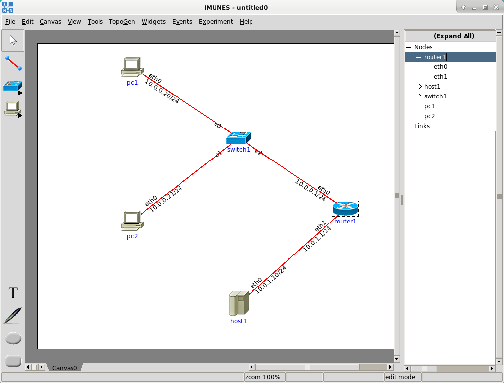
Network elements configuration parameters can be also changed through the topology tree. To show the topology tree turn on the Show Topology Tree option from the View menu. The tree with a list of network topology elements (nodes and links) will be shown on the right side of the window (Figure 4.5). To open the network element configuration window double click or use the Enter keyboard button on node, interface or link label in the topology tree.

Figure 4.5: Changing configuration parameters through the topology tree

Depending on the type of a network element in our topology, there are 4 types of configuration windows:

• Hub/LAN switch configuration window
• PC/Host/Click router configuration window
• Router configuration window
• Link configuration window

There are also other types of configuration windows which are explained in other sections:

• External interface configuration window
• External connection configuration window
• NAT64 configuration window
• RSTP switch configuration window
• Filter node configuration window
• Packet generator configuration window
• Click switch configuration window

4.1.2.1 Hub/LAN switch configuration window

The hub/LAN switch configuration window, as well as the configuration windows of other node types, contains a node name field. Besides that it contains only link layer interface parameters.

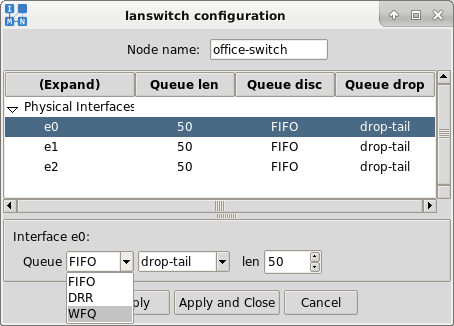
We will change the LAN switch name and data packet scheduling method (from preconfigured First In First Out (FIFO) data packet scheduling method to Weighted Fair Queuing (WFQ) method).

Change the node name to office-switch. To change data packet scheduling method select the link layer interface e0 from the list of interfaces, choose WFQ option from the Queue menu and click on the Apply button (Figure 4.6).

Figure 4.6: LAN switch configuration window

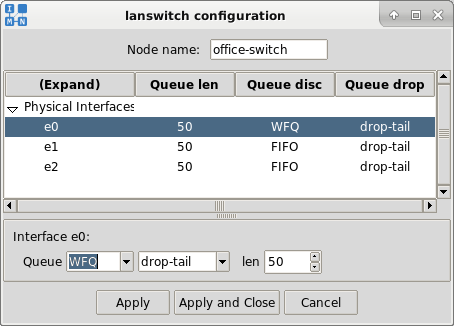
Packet scheduling method is now applied and you can see new queuing discipline for interface e0 in the column Queue disc (Figure 4.7).

Figure 4.7: LAN switch configuration window with applied changes

Repeat the same procedure for the other link layer interfaces. Changed configuration is already applied so you can close the configuration window with the Cancel button but you can also use the Apply and Close button.

4.1.2.2 PC/Host/Click router configuration window

The PC/Host/Click router configuration window consists of two subwindows. Each of them is associated with one of the following tabs: Configuration and Interfaces (Figure 4.8).

Figure 4.8: Tabs in the PC/Host/Click router configuration window

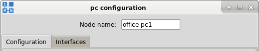
Besides a node name field, PC/Host/Click router configuration window contains startup services, routing parameters and custom configuration parameters (in the window associated with the Configuration tab) and network interface parameters (in the window associated with the Interfaces tab).

We will change the node name, network interface parameters and routing parameters.

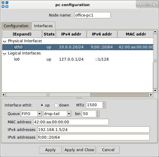
Change the host node name to office-host and PC node names to office-pc1 and office-pc2. To change IPv4 address left click on the Interfaces tab, select interface eth0 from the list of interfaces, change the IPv4 address field and click on the Apply button (Figure 4.9). We will change the host IPv4 address field to 192.168.2.5/24 (now it belongs to 192.168.2.0/24) and PC IPv4 address fields to 192.168.1.5/24 and 192.168.1.7/24 (now they belong to network 192.168.1.0/24). IP address fields require the CIDR notation, so the IPv4 address is followed by a slash and a network length.

Figure 4.9: Changing IPv4 address

4.1.2.2.1 Static routes

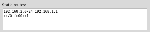
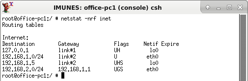
PCs and Hosts both use static routing. The preconfigured routing table contains only the default route. Every static route, as well as the default route, consists of:

1. the destination network: an IP address which is followed by a slash and a network prefix and
2. the next hop network interface IP address (which is an IP address without a slash and without a network prefix).

If the route syntax is wrong, that route will be silently ignored.

We will add the static route on office-pc1 and office-pc2 for the network 192.168.2.0/24 through the gateway 192.168.1.1 (Figure 4.10).

Figure 4.10: Adding the static route on the PC

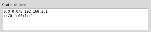
On office-host we will change default gateway address to 192.168.2.1 (Figure 4.11).

Figure 4.11: Adding the static route on the PC

IPv6 addresses and default routes (placed below IPv4 addresses and routes) can be deleted.

To apply the changed configuration and close the configuration window click on the Apply and Close button.

4.1.2.3 Router configuration window

The router configuration window, in addition to fields from PC/Host/Click router configuration window, contains the part for choosing the routing model and protocols, as well as an IPsec tab with IPsec parameters (See IPsec Section TODO).

We will only change the node name and network interface parameters.

Change the node name to office-router and IPv4 addresses on both network interfaces: 192.168.1.1/24 on the network interface eth0 and 192.168.2.1/24 on the network interface eth1.

4.1.2.3.1 Routing models and protocols

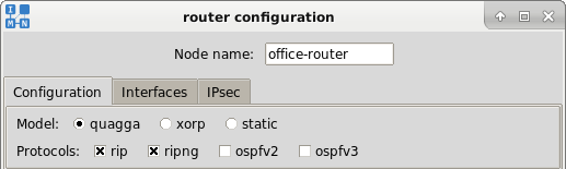
There are three possible routing models:

1. the quagga model
2. the xorp model (eXtensible Open Router Platform)
3. the static model

In the case of quagga and xorp routing models, there are options for enabling/disabling RIP, RIPng, OSPFv2 and OSPFv3. By default, all new quagga or xorp router instances will have both RIPv2 and RIPng enabled. The defaults can be changed with the Tools $\to$ Routing protocol defaults option from the menubar, which will be applied to all selected routers (if any) at the time of change, as well as to all the subsequentially created ones (see Section 5.3.5). In the case of static routing model, the router uses routes from the static routes field that has the same syntax as the static routes field in the PC/Host/Click router configuration window.

We will leave the default router model - quagga with RIP and RIPng protocols enabled, and OSPFv2 and OSPFv3 protocols disabled (Figure 4.12).

Figure 4.12: Routing models and protocols

4.1.2.4 Link configuration window

The link configuration window offers the possibility to configure the link bandwidth (between 0 and 10⁹ bps), the propagation delay (between 0 and 10⁷ $\mu$s), the bit error rate (between 0 and 10¹²) and the probability of package duplication (between 0 and 50%). There are also display properties: the link width (line thickness between 1 and 8) and the link color (red, green, blue, yellow, magenta, cyan or black).

Figure 4.13: Link configuration window

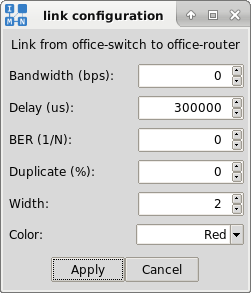
Default values are as follows: the link which transmits packets without errors and without any possibility for the packet duplication with the unlimited link bandwidth and the zero propagation delay. The link width is set to value 2 and the link color is red.

We will leave default values on all links except on the link between office-switch and office-router (Figure 4.14). On that link we will set up the delay of 30000 $\mu$s. Delay will be tested during the network simulation with the traceroute tool (see Section 4.1.3).

4.1.2.5 Configured network topology

Configured network topology should look like the one in Figure 4.14.

Figure 4.14: Configured network topology

4.1.3 Simulating a simple network

4.1.3.1 Starting an experiment

After the network topology is completely built and properly configured, we will start an experiment with the Experiment $\to$ Execute option from the menubar and IMUNES will switch from the edit mode to the execute mode. In the process of starting an experiment, IMUNES creates and configures the virtual network. That will take a few seconds and all events during that process will be shown in the statusbar placed at the bottom of the window.

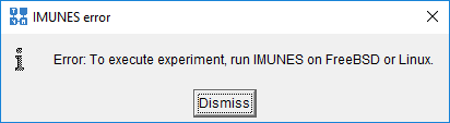
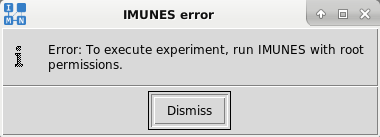
NOTE: Although you can draw network topology on any system that supports Tcl/Tk (Linux, FreeBSD, Windows, Mac OS X, Solaris), an experiment can only be started on FreeBSD and Linux operating systems with root permissions (Figure 4.15 and Figure 4.16)!

Figure 4.15: Starting an experiment in Windows

Figure 4.16: Starting an experiment in FreeBSD without root permissions

In addition to configured parameters, each node will be set with the loopback interface, a router will have the kernel forwarding enabled, and a host node will have portmap and inetd started.

Information about the time spent instantiating the network topology is shown in the statusbar (Figure 4.17).

Figure 4.17: Message about the instantiation of the network topology

In the right corner of the statusbar you can also see that IMUNES now works in the execute mode, as well as experiment unique identifier.

4.1.3.2 Options from the node and the link menu

To open the node menu in the execute mode right click on the node. Note that the menu in the execute mode is different from the menu in the edit mode. It offers the possibility to select the node connected to this node (Select adjacent), to see the current configuration (Configure), to Start / Stop / Restart the network element, to start / stop / restart any of the possible Services or to Import Running Configuration from the Settings menu. The Import Running Configuration option copies the current MTU value and IPv4/IPv6 addresses from the running node to its configuration. It is also possible to open the Shell window (X terminal with a Unix shell), Wireshark or tcpdump network sniffers on any of the interfaces, Firefox Web Browser or a Mail client.

Figure 4.18: Network-layer node menu in the execute mode

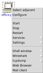
Note that both the node and the link menu in the execute menu offer the possibility to open the configuration window (Configure label).

From the node configuration window in the execute mode it is possible to change only the node name. Other node parameters such as link layer interface parameters, network interface parameters and routing parameters can be changed from the shell window on each node. To change those parameters from the node configuration window, stop the node (using the Stop label), change parameters and then start the node agin (using the Start label).

On the other side, from the link configuration window in the execute mode it is possible to change the following link parameters: link bandwidth, the propagation delay, the bit error rate and the probability of package duplication. It is also possible to change display properties: the link width and the link color.

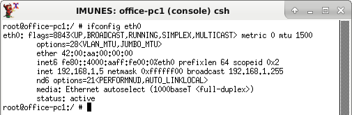
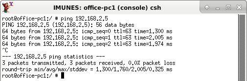
We will now check if the virtual network topology is properly configured. Open the shell window (e.g. Shell window $\to$ csh or simply double click on the node) on the network element (e.g. office-pc1).

• To check the network interface eth0 parameters type the following command: ifconfig eth0. The result is shown in Figure 4.19.

  Figure 4.19: Shell window on office-pc1, network interface parameters

  
  
  

  

• To check static routes type the following command: netstat -nrf inet. The result is shown in Figure 4.20.

  Figure 4.20: Shell window on office-pc1, static routes

  
  
  

  

• To test if a particular network element is reachable (e.g office-host) type the following command: ping 192.168.2.5. The result is shown in Figure 4.21. To stop transmitting packets press Control-C keyboard button.

  Figure 4.21: Shell window on office-pc1, pinging office-host

  
  
  

  

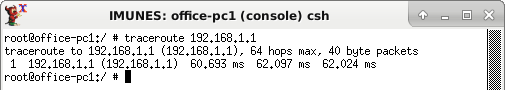
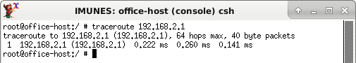
We will test delay on the link between office-switch and office-router, which is set to 30000 $\mu$s (30 ms), by using the traceroute tool:

• In the shell window on office-pc1 type the following command:
  traceroute 192.168.1.1. The result is shown in Figure 4.22.

  Figure 4.22: Shell window on office-pc1, traceroute to office-router

  
  
  

  

• In the shell window on office-host type the following command:
  traceroute 192.168.2.1. The result is shown in Figure 4.23.

  Figure 4.23: Shell window on office-host, traceroute to office-router

  
  
  

  

4.1.3.3 Terminating an experiment

To terminate an experiment and switch from the execute mode to the edit mode use the Experiment $\to$ Execute option from the menubar. During the termination process, IMUNES will terminate active services on each node and shut down all network elements (links and nodes with both virtual and physical interfaces). The termination is finished when the message about the successful cleanup shows up in the statusbar (Figure 4.24).

Figure 4.24: Message about the successful cleanup

4.2 Configuration files management

4.2.1 Saving a virtual network configuration

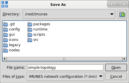
After the virtual network is successfully built, configured and tested, it can be saved with File $\to$ Save or File $\to$ Save As options from the menubar. The virtual network topology is saved in IMUNES network configuration file format (.imn).

Figure 4.25: File Save dialog

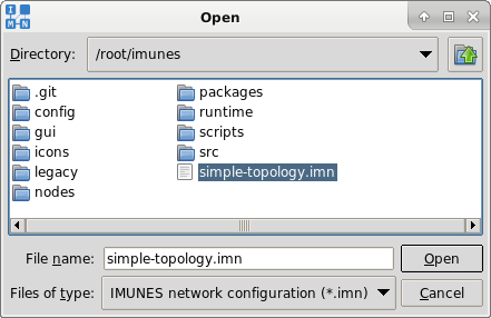
The structure of the configuration file is simple and suitable for changing with a text editor (see Appendix 8).

4.2.2 Opening a virtual network configuration

To open an existing IMUNES network configuration file use the File $\to$ Open option from the menubar and select it from the invoked File Open dialog.

Figure 4.26: File Open dialog

The other way to open an imn file is to start IMUNES with that file as an argument: imunes simple-topology.imn