Next: 6. Installation Up: IMUNES manual Previous: 4. Quick Intro
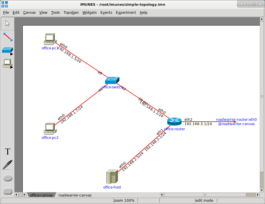
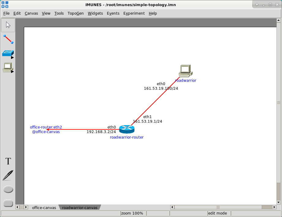
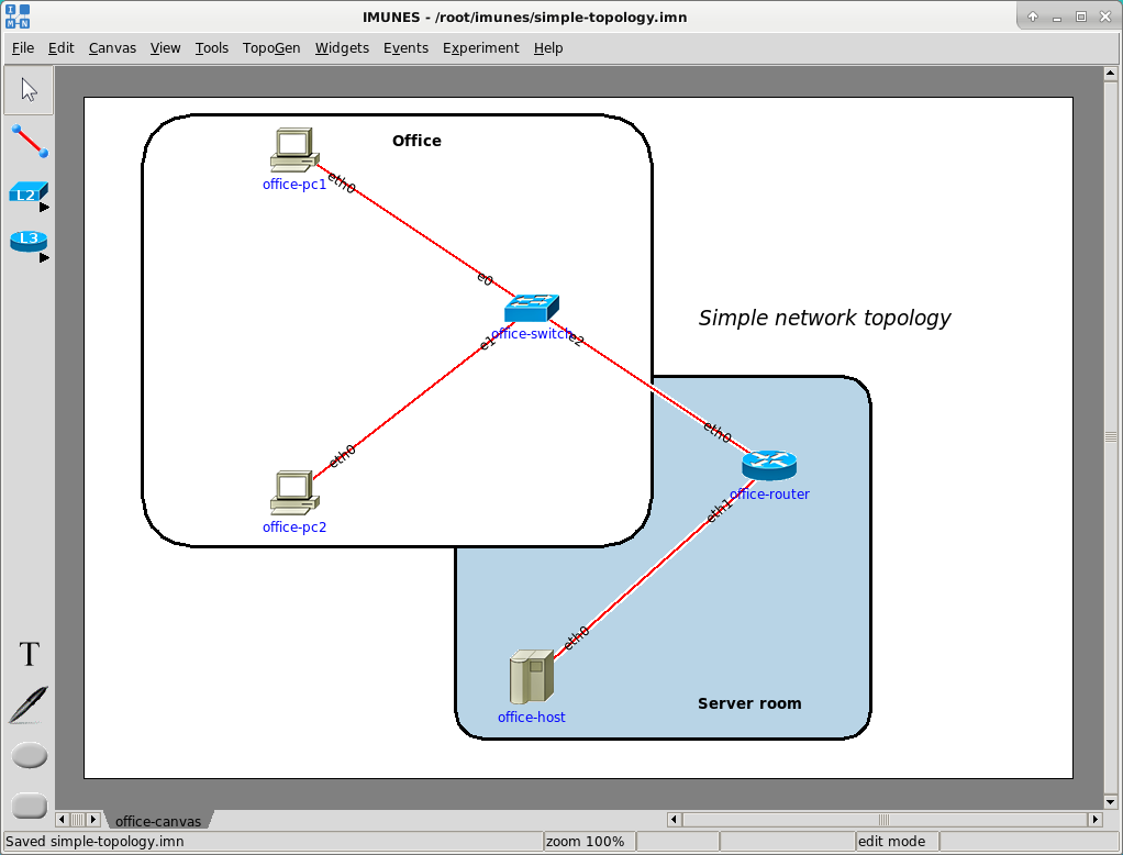
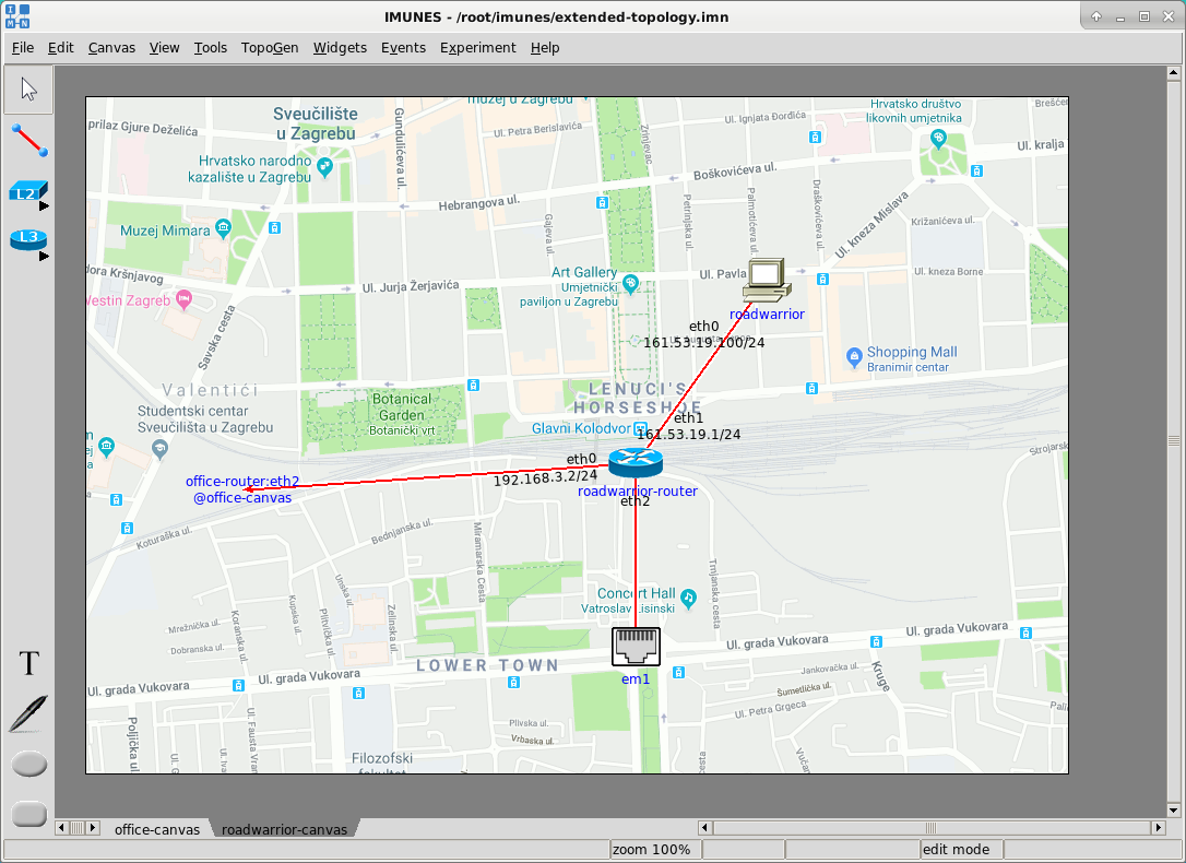
The simple network topology is placed in the office-canvas while the additional elements are placed in the roadwarrior-canvas. The roadwarrior-canvas consists of a router (roadwarrior-router), a PC (roadwarrior) and a physical interface. The roadwarrior-router is connected to the office-router on the office-canvas through the 192.168.3.0/24 network, the PC is in the 161.53.19.0/24 network whereas the physical interface is in the 161.53.20.0/24 network.
We will now extend the simple network from the last chapter by adding the
roadwarrior-router, roadwarrior and the physical interface all
placed on another canvas. To open an existing IMUNES network configuration file
use File ![]() Open from the menubar or start IMUNES with the imn file
as an argument: imunes simple-topology.imn. Check that you are in the
edit mode. If not, switch with Experiment
Open from the menubar or start IMUNES with the imn file
as an argument: imunes simple-topology.imn. Check that you are in the
edit mode. If not, switch with Experiment ![]() Terminate.
Terminate.
Canvas management consists of two main elements:
To add a new canvas use the Canvas ![]() New option from the menubar or
double click on the empty space in the canvas tabs list at the bottom of the
window.
New option from the menubar or
double click on the empty space in the canvas tabs list at the bottom of the
window.
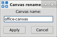
You can rename the canvas with the Canvas ![]() Rename option from the
menubar or double click on the canvas tab in the canvas tabs list. (Figure
5.2) Similarly the Canvas
Rename option from the
menubar or double click on the canvas tab in the canvas tabs list. (Figure
5.2) Similarly the Canvas ![]() Delete option
deletes the active canvas.
Delete option
deletes the active canvas.
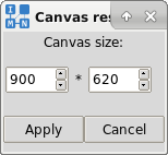
There is also the option Canvas ![]() Resize that allows you to define a
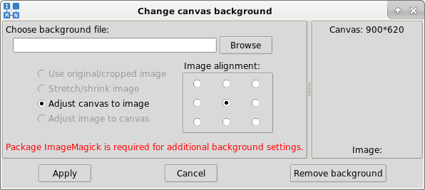
custom canvas size in pixels. The default canvas size is 900*620 pixels.
(Figure 5.3)
Resize that allows you to define a
custom canvas size in pixels. The default canvas size is 900*620 pixels.
(Figure 5.3)
Canvas selection can be done with the options from the Canvas menu (Previous, Next, First, Last) or simply by clicking the tab with the canvas name on it.
Rename the existing canvas Canvas0 into office-canvas. Add a new canvas, rename it into roadwarrior-canvas and select it as the active canvas.
This canvas is empty so we will add a router by selecting the router tool and
clicking on the empty canvas. Rename this router into
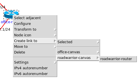
roadwarrior-router. Switch to the office-canvas. Now we will
connect the office-router and the roadwarrior-router. To do that,
right click on the office-router and select Create link to ![]() roadwarrior-canvas
roadwarrior-canvas ![]() roadwarrior-router option (Figure
5.4) from the popped up menu. This will create a link
between roadwarrior-router and office-router.
roadwarrior-router option (Figure
5.4) from the popped up menu. This will create a link
between roadwarrior-router and office-router.
On the office-router set the eth2 interface IPv4 address to 192.168.3.1/24. On the roadwarrior-router set the eth0 interface IPv4 address to 192.168.3.2/24. We will add another PC to the roadwarrior-canvas, name it roadwarrior and connect it with the roadwarrior-router. On the roadwarrior set the eth0 IPv4 address to 161.53.19.100/24. On the roadwarrior-router set the eth1 IPv4 address to 161.53.19.1/24.
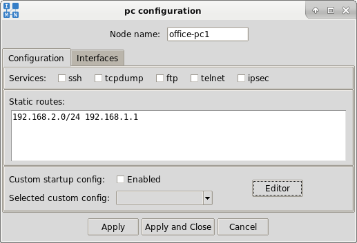
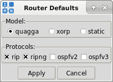
The roadwarrior-router uses the same dynamic routing model (quagga) as the office-router and we do not need to configure anything else on the router. The roadwarrior uses static routes and we will need to change the default route gateway in static routes field of the roadwarrior configuration window to 0.0.0.0/0 161.53.19.1.
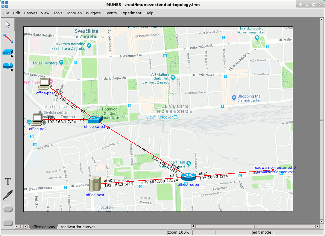
Finally, the configured network topology should look like the following (Figure 5.5 and Figure 5.6):
Both the roadwarrior and roadwarrior-router can be easily moved
from roadwarrior-canvas to office-canvas with the Move To
![]() office-canvas from the node menu. The link between
roadwarrior-router and office-router, as well as any other link,
can be deleted with the Delete option from the Link menu. To open
the link menu, use the right click on the link and choose the
Delete option.
office-canvas from the node menu. The link between
roadwarrior-router and office-router, as well as any other link,
can be deleted with the Delete option from the Link menu. To open
the link menu, use the right click on the link and choose the
Delete option.
When we are done with network configuration, we can start the experiment with
Experiment ![]() Execute from the menubar. We can now check that the
roadwarrior can ping both networks (192.168.1.0/24, 192.168.2.0/24) and
additionally, that the network 192.168.1.0/24 does not have an access to the
roadwarrior, but it has access to the 192.168.2.0/24 network.
Execute from the menubar. We can now check that the
roadwarrior can ping both networks (192.168.1.0/24, 192.168.2.0/24) and
additionally, that the network 192.168.1.0/24 does not have an access to the
roadwarrior, but it has access to the 192.168.2.0/24 network.
The External interface tool from the toolbox provides the possibility to attach a physical interface to a virtual node. This way the virtual network is able to communicate with nodes from the external network.
We will now add the external interface to the roadwarrior-canvas. To add a external interface to the canvas select the External interface tool and click on the canvas.
External interface nodes can be connected either with the LAN switch or the router. Connect the newly created external interface with the virtual node roadwarrior-router using the Link tool from the toolbox or the Create link to option from the node menu.
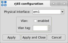
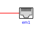
The newly created external interface node is unassigned and in the node name field it contains UNASSIGNED. Open the external interface configuration window with a double click or right click on it and select the Configure option. Choose the name of the designated physical interface in the Physical interface drop-down list, e.g. em1, obtained from ifconfig -a command ran on the physical machine (outside IMUNES). (Figure 5.7) The name of the physical interface will appear in the node name label. It is also possible to assign a VLAN tag to it. (Figure 5.8)
Check that roadwarrior-router has a properly configured IP address on the network interface connected to the physical interface. Additionally, check that routes which route packets between virtual network and the external network through the physical interface exist in both the external network and in the virtual network (on roadwarrior-router).
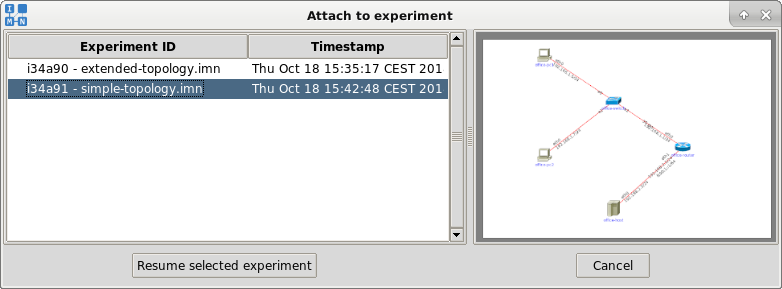
Save this configuration to a new file by selecting the Save as option from the File menu. Name the file extended-topology.imn.
To attach to the you can double-click it's entry or use the Resume selected experiment button.
The configuration window of each network layer node (PC, Host, Router, NAT64 and Click router) also has the Custom startup configuration field. In order to view or edit the generated startup configuration click on the Editor button as shown in Figure 5.10.
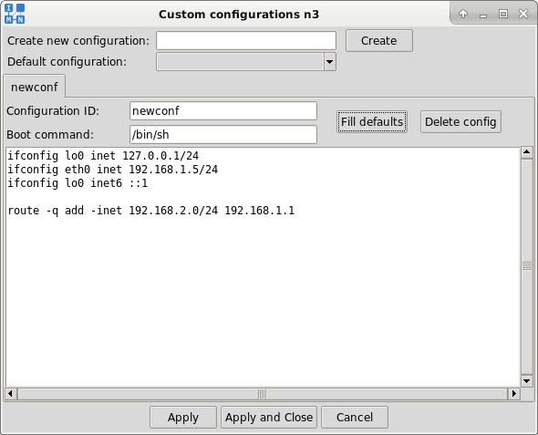
In a newly opened window, write a new configuration name and click Create. An empty configuration file will be created. By clicking on Fill defaults, in case of a non-router network layer node or a router node with the static routing model, the default configuration consists of ifconfig and route commands with the /bin/sh shell. Figure 5.11 shows the created default configuration.
It is possible to add custom commands that will be executed at the boot time. When finished, click on the Apply or Apply and Close button to save the changes. When you have multiple configurations, you can choose the default one in the Default configuration drop-down menu. To delete a configuration, select its tab and click Delete config button.
NOTE: After starting the network simulation, the new/custom configuration will be considered only if Custom startup configuration is enabled. This is done by checking the Enabled check box in the Custom startup config field in Figure 5.10.
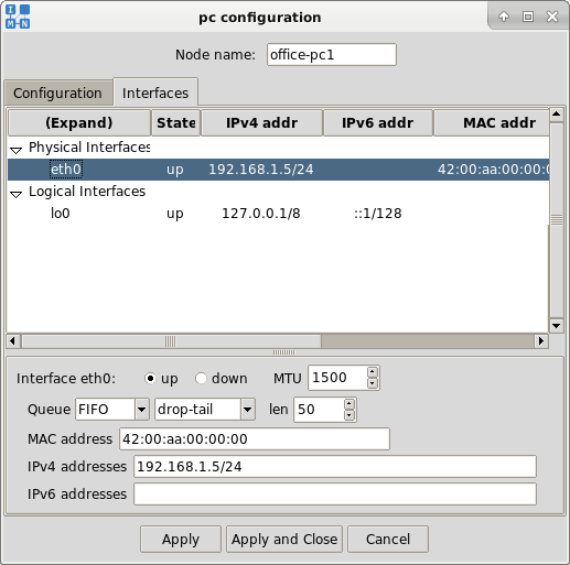
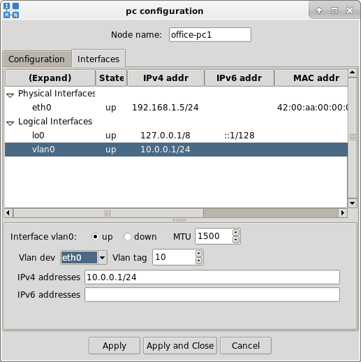
When the Interfaces tab is opened, a configuration window similar to the one shown in Figure 5.12 is shown to the user. The Physical Interfaces list represents actual interfaces connected to links in IMUNES. Thus we can see that the selected node has one link in IMUNES.
IMUNES also offers the feature to configure additional logical interfaces. By default only one logical interface is added: lo0 - the loopback interface with the following addresses: 127.0.0.1 for IPv4 and ::1 for IPv6.
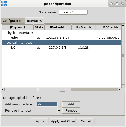
Users can configure additional logical interfaces by clicking on the Logical Interfaces item in the Interfaces list. The Logical Interfaces configuration window is show in Figure 5.13. At the moment IMUNES supports two types of logical interfaces: lo and vlan.
Figure 5.14 shows an example for setting up a vlan logical interface vlan0 on a physical interface eth0 with an arbitrary tag 10 and an IPv4 address 10.0.0.1/24.
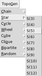
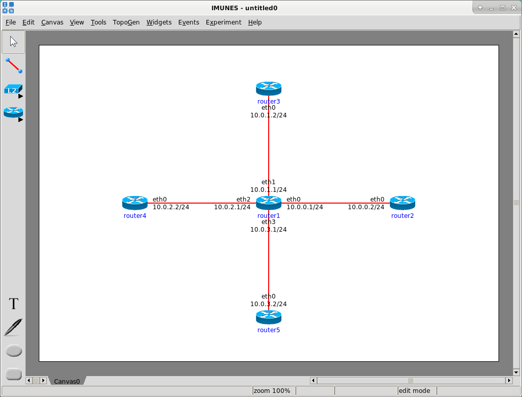
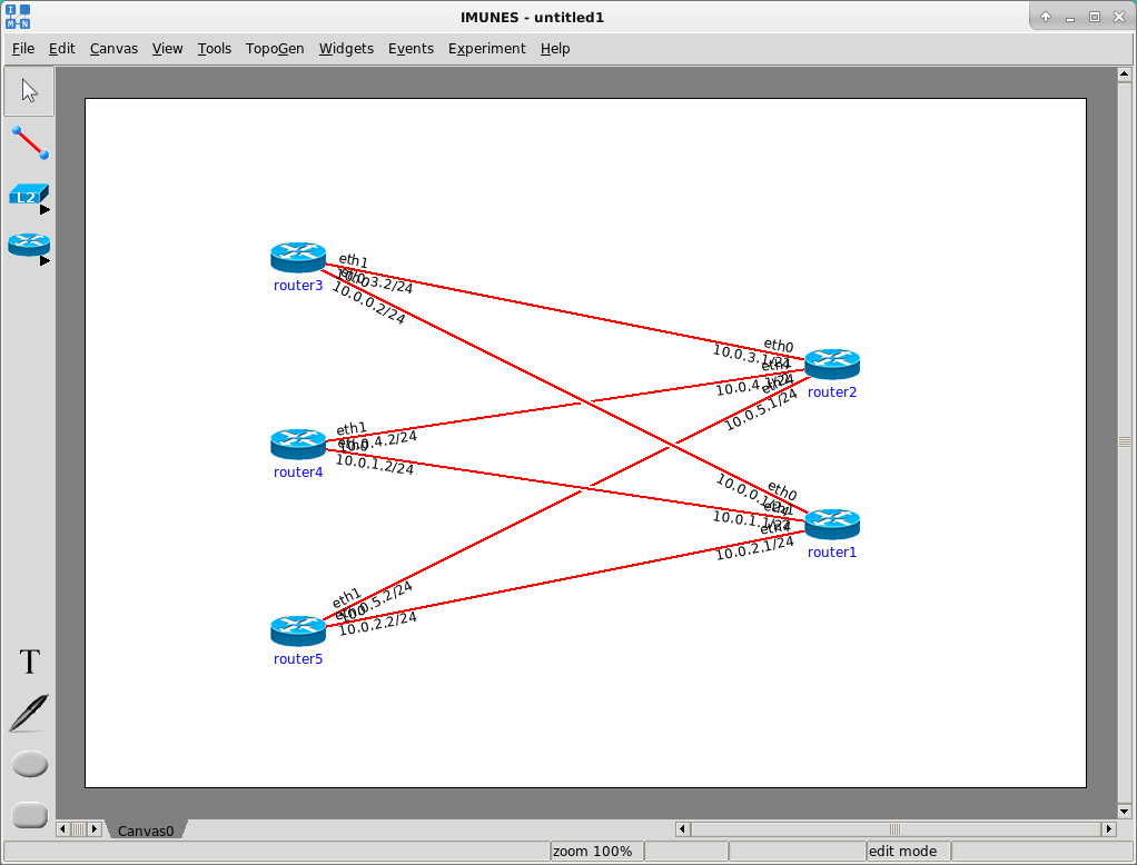
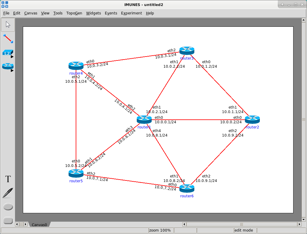
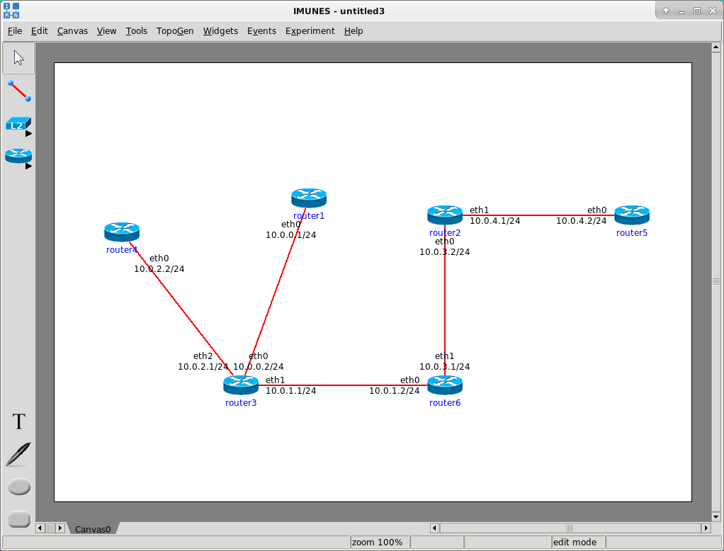
Some examples can be seen in Figure 5.17, Figure 5.18 and Figure 5.19. In order to generate a topology first select the network layer nodes (router, host or PC) from the toolbox and then the desired topology type e.g. bipartite graph K(2,3) (see Figure 5.18).
In case of random topology an additional information is needed, so beside the number of the nodes it is also necessary to specify the number of links. The nodes in the random topology will be randomly connected with the number of links specified before. An example of generating a random topology:
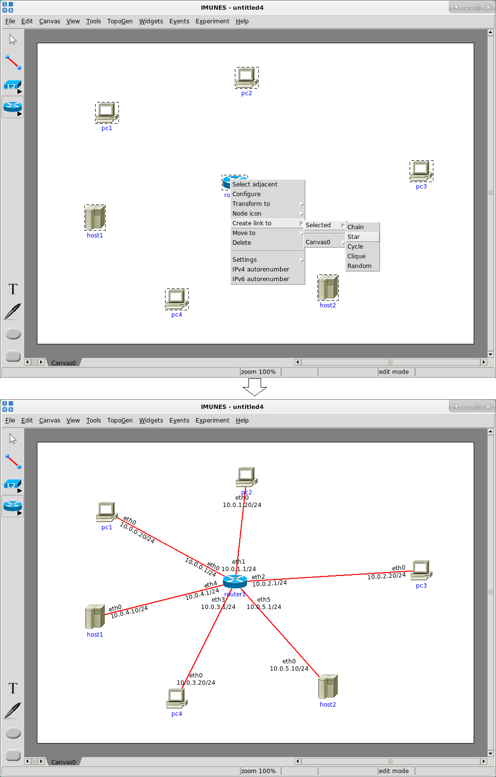
Using the TopoGen tool you can generate topologies containing one type of node (router, host or PC). In that case, new nodes of the same type are created and placed on the canvas. Another option is to add new nodes to canvas and then connect them using the topology generator:
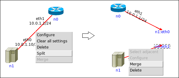
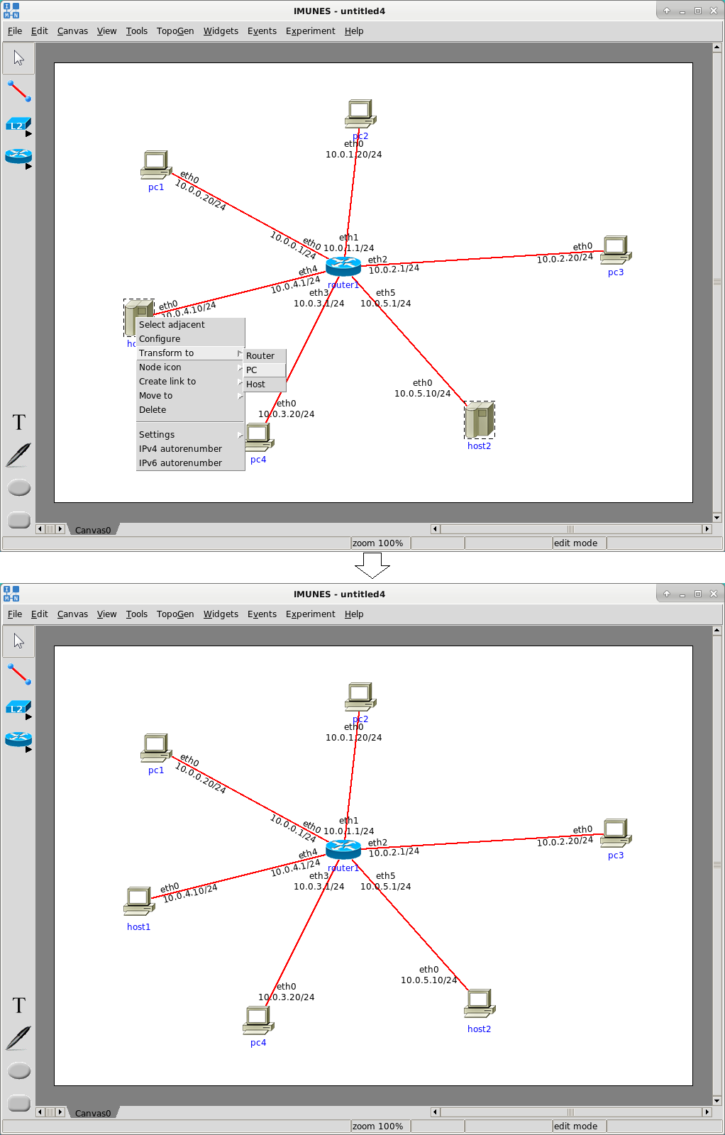
In addition to that, it is also possible to transform existing nodes:
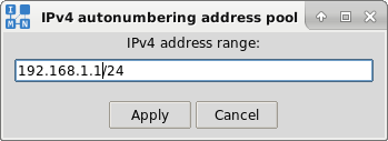
In order to replace default 10.0.0.0/24 address pool, set variable-mask IPv4 address pool through the invoked dialog. CIDR notation is required, so the IPv4 address needs to be followed by a slash and a network length. To apply changes click on the Apply button. The given address pool will be applied to all the subsequentially created network layer elements (Figure 5.24).
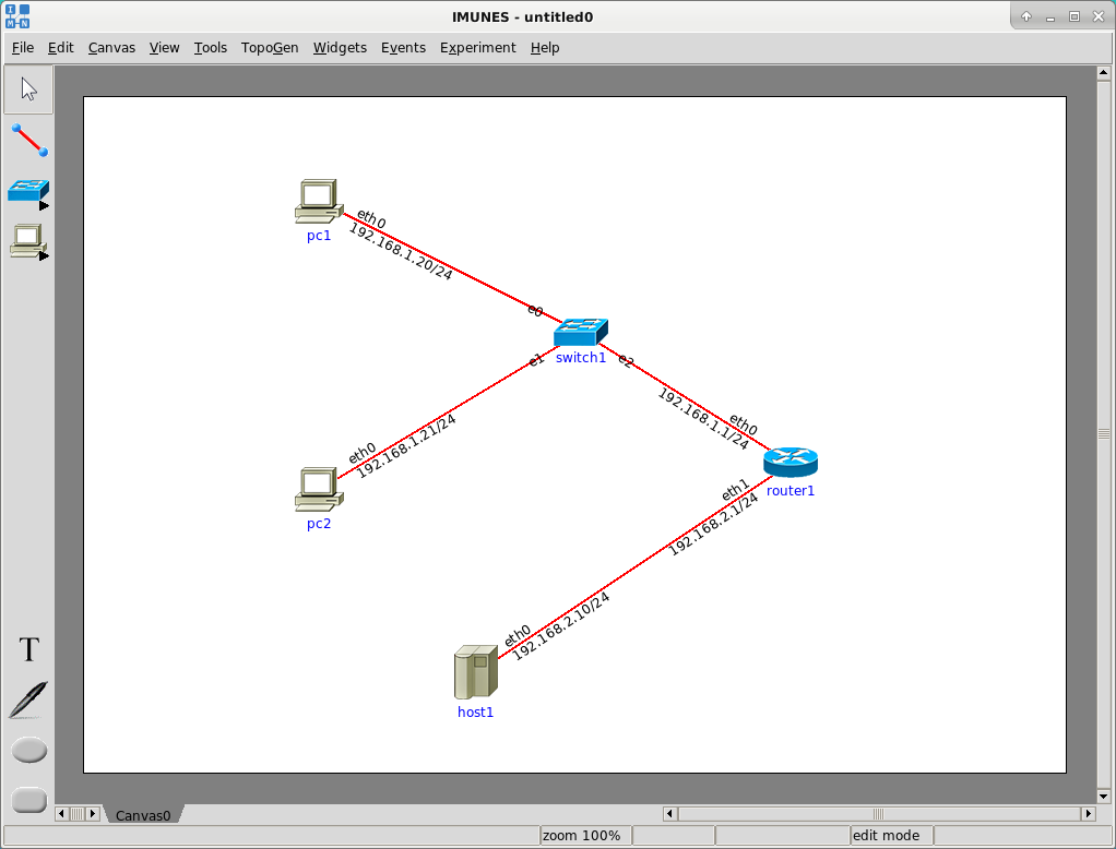
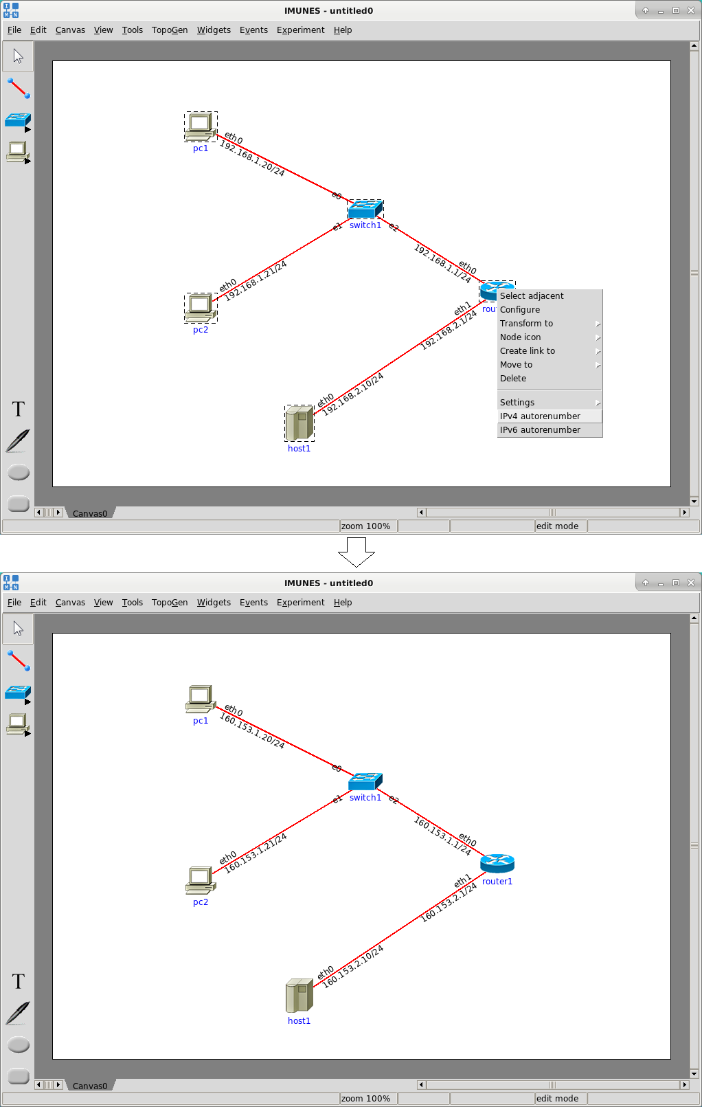
In order to apply the given address pool to selected elements, right click on the network layer element and choose the option IPv4 autorenumber from the popped up menu. In example shown in Figure 5.25 we have set IPv4 address pool to 160.153.1.1/24, selected all network elements and selected the option IPv4 autorenumber from the node menu to apply the given address pool to selected elements.
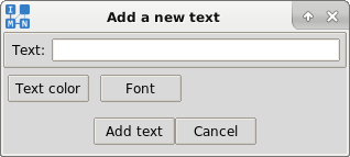
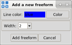
To add an annotation to the canvas, select the appropriate tool and click (and drag) where you want to add the annotation. A popup window will be shown. There you can define how will the annotation look.
When created, annotations can be moved around on the canvas. This is done by using the select tool. Click on the annotation and then drag it to its destination.
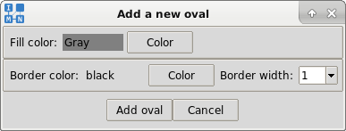
The oval annotation lets you define the following additional options (Figure 5.33):
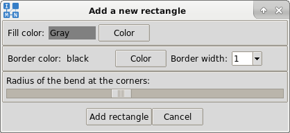
The rectangle annotation lets you define the following additional options (Figure 5.34):
Example of the annotations usage is shown in Figure 5.35.
The options for changing the canvas background image are accessible through the Canvas and View menu and through the menu that is opened with a right click on the empty canvas (Figure 3.6 and Figure 5.36).
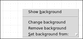
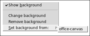
All options related to the canvas background are accessible in the Background image menu (Figure 5.36):
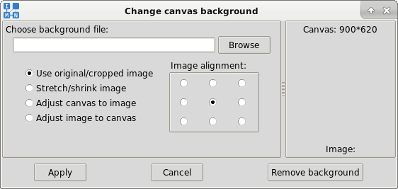
To set a canvas background you need to open the Change canvas background window (Figure 5.37).
This window is divided into two main parts:
When the image is selected there are four image setting modes that can be chosen:
We will use the extended topology example (extended-topology.imn) to set
canvas background images. On the office-canvas we will set a background
image. Then we will go to the roadwarrior-canvas and set that same image
using the Set background from ![]() office-canvas option (Figure
5.39).
office-canvas option (Figure
5.39).
The final result is shown in Figure 5.40 and Figure 5.41.
The Change node icons option opens the Set custom icon window (Figure 5.43).
This window is divided into two main parts (Figure 5.43):
We will now open the extended-topology.imn file and set a custom icon. We will choose the library icon ipfirewall.gif for the roadwarrior-router. The final result is shown on Figure 5.44.
Let's take the simple-topology.imn example and set the icon size to small. (Figure 5.46)
Currently, only two sizes are available, normal and small. Otherwise, custom icons can be used.
The event scheduler supports two general classes of schedulable events: one-time changes and periodic functions.
One-time events update the selected parameter at requested point in time, leaving that parameter constant throughout rest of the experiment execution, or until another event updates it to a new value at some later point in time.
Periodic functions allow for time-variant functions to be applied to selected parameters by specifying those functions as single events. Subsequently scheduled events acting upon the same parameter will cancel the current periodic function and replace it with either a constant value or another periodic function.
Each event entry occupies a single line of text, consisting of four fields: deadline, target parameter, function and function parameters. The first field, deadline, is specified as an integer number of seconds since experiment instantiation. The second field, target parameter, may be one of the following: bandwidth, delay, ber, duplicate, width or color. The remainder of the line is further parsed as a function. The type of the function is determined by the leading keyword, which may be either const, ramp, rand or square. When saving the configuration through the events editor a syntax check will be performed. If the syntax is wrong the configuration will not be saved and a popup dialog will show the first line that has a syntax error.
At t = 30 s, bandwidth of the selected link will be set to 128 Kbps, and will continue to grow at a rate of 8 Kbps each 2 s.
Also at t = 30 s, the delay will begin assuming a random value between 80 ms and 120 ms, and will continue to change the setting to new random values in the same range each 8 s.
At t = 60 s, the delay will cease to assume random values, and instead it will begin to oscillate between two discrete values, 100 ms and 200ms, each 10 s.
Also at t = 60 s, the bit error rate (BER) will be set to 1, resulting in all frames traversing the link to be silently dropped.
At t = 90 s, the BER is reset back to 0, allowing for all frames to traverse the link without artificial losses.
At t = 120 s, the oscillation of the delay parameter will stop, and delay will be reset to 0 ms for the rest of the experiment execution time.
The current time is shown on the status bar after the zoom value. (Figure 4.17)
IMUNES experiments are defined via plain-text configuration files, which currently describe virtual nodes and links, as well as additional objects related only to GUI visual properties and annotations. The other way to configure events is manual editing of an existing configuration file.
The example bellow shows a configuration section describing a virtual link in an IMUNES experiment. The link l0 connects virtual nodes n0 and n1, has the bandwidth constraint set to 128 Kbps, and has the thickness of the line representing the link in the GUI set to 6 pixels. All of the mentioned properties are directly controllable via the IMUNES GUI. The configuration for link l0 also includes an empty placeholder for schedulable events, meaning that no events have been programmed for this link.
The events section in the configuration file accepts the same commands as does the Events editor in the GUI.
# imunes -b simple-network.imn
Using IMUNES through GUI, the Experiment![]() Terminate option is used
for shutting down the simulation and cleaning up the virtual network topology
from the kernel. The CLI alternative for the latter is the following command:
Terminate option is used
for shutting down the simulation and cleaning up the virtual network topology
from the kernel. The CLI alternative for the latter is the following command:
# imunes -b -e experimentId
The parameter exeperimentId represents the experiment identifier. In order to get the experiment identifier you can use the himage command. With himage -l you will get a list of identifiers of all started experiments.
Two main commands exist in FreeBSD for manging and configuring previously created jails:
A virtual image or vimage is a jail with its own independent network stack instance. Every process, socket and network interface present in the system is always attached to one, and only one, virtual network stack instance (vnet). During system bootup sequence a default vnet is created to which all the configured interfaces and user processes are initially attached.
The jexec command allows for execution of arbitrary processes in a targeted virtual image.
jexec jname command ...
The jexec command starts the selected command and it's arguments in the jail jname.
To find out the names of started jails the jls command is used:
jls [-hnqsv] [parameter ...]
Since the default jls command doesn't list names of jails a better output is provided using the command:
jls -h jid name host.hostname
Also, the command jls -v gives a more detailed output.
Execute the ifconfig command in the jail with the jail name n1:
# jexec n1 ifconfig
Execute the csh command in the IMUNES virtual node named host1:
First we need to find out the jail ID or jail name to execute the wanted command:
# jls -h jid name host.hostname | grep host1
The first parameter output is the jail ID, the second is the jail name and the last is the hostname. To execute the command you need the jail ID or jail name:
# jexec jid csh
# jexec jname csh
IMUNES comes with the himage tool that enables the usage of hostnames when starting commands in virtual nodes. The himage tool starts the jexec command with the appropriate jail name so that the user doesn't have to search for it.
The himage command has the following options:
Example of usage of the command himage on a node with the hostname "pc" to get a list of running processes:
# himage pc ps ax
If there are multiple experiments running and there are nodes with the same hostnames in these experiments the himage command accepts the following node specification where vi_hostname is specified as hostname@eid, where eid is the experiments' ID.
# himage hostname@eid command ...
i.e:
# himage pc@i3d05a ps ax
where i3d05a is the experiment ID of the running experiments. To find out which experiments are running the himage -l command can be used as well as jls -h jid name host.hostname.
Execute the ifconfig command the IMUNES node named server:
# himage server ifconfig
While the himage command is used for running programs inside virtual nodes the hcp is used to copy files directly to the filesystem of running mobile nodes, thus simplifying deployment of configuration files for starting various services on virtual nodes.
Usage of the command hcp:
hcp [cp_command_options] [vi_hostname1:]filename [vi_hostname2:]filename
The hcp command invokes the cp command with the specified options. If the vi_hostname1 is specified the script copies a file from the virtual node, otherwise it copies a file from the local folders. The second vi_hostname2 specifies on which node the first file will be copied, if not specified the file is copied to the local folders.
vi_hostname is specified in the same way as in the himage command, hostname or hostname@eid.
Copy file dhcpd.conf from a local folder to the virtual node DHCP:
# hcp dhcpd.conf DHCP:/usr/local/etc/
Copy file message.txt from the virtual node PC to a local folder:
# hcp PC:/root/message.txt .
Copy file index.html from the virtual node HOST to the virtual node HTTP:
# hcp HOST:/usr/local/www/data/index.html HTTP:/usr/local/www/data/
This is an example of starting an DHCP server through a script with the provided configuration file dhcpd.conf.
Kill the server if it's started:
# himage DHCP killall -9 dhcpd
Copy the configuration file:
# hcp dhcpd.conf DHCP:/usr/local/etc/
Create the .leases file defined in dhcpd.conf:
# himage DHCP touch /var/db/dhcpd.leases
Start the sever with the copied configuration file:
# himage DHCP dhcpd -cf /usr/local/etc/dhcpd.conf
The vlink tool is used to change link parameters. The following link parameters are available:
A link is identified by the endpoint node names. The link between pc1 and pc2 is identified by pc1-pc2 or pc2-pc1.
Usage of the command vlink:
vlink [options] link_name[@eid]
Setting the bandwidth to 10 Mb/s with a delay of 30 ms to the link connecting router1 and pc1:
# vlink -bw 10000000 -dly 30000 router1:pc1
Generate an error on one bit in a million:
# vlink -BER 1000000 router1:pc1
Set packet duplication to 20 # vlink -dup 20 router1:pc1
Modifying a link in a specific experiment (i.e. Experiment ID = i56ad1):
# vlink -dup 20 router1:pc1@i56ad1
To reset the link settings to the default values the -r flag is used:
# vlink -r router1:pc1@i56ad1